"What is the lasso regression? Add L2 norm into loss function."

Norm is a commonly used concept in mathematics, which is also often encountered in machine learning.

The first thing that needs to be clear is that Norm is a function. We usually use it to measure the value of the vector in machine learning. The norm is defined as:

$\|x\|_p = \left(\sum_{i=1}^m |x_i|^p\right)^{1/p}$

Common Norm:

1. $L^2$ Norm:
   When p is 2, $L^2$ Norm is also called Euclidean norm. It represents the distance from the original to the points determined by the vector x. It is applied very frequently in machine learning.

   $\|x\|_2 = \left(\sum_{i=1}^m |x_i|^2\right)^{1/2}$

2. Square $L^2$ Norm:
   It is square of $L^2$ norm, $ |x|_2^2$. The advantage is that it is obviously easier to calculate, which can be simply calculated by the dot product of $X^TX$.

3. $L^1$ Norm:
   In some case, $L^2$ Norm is not very popular, because it grows very slowly near the origin. Sometimes, it is important to distinguish elements that happen to be zero and non-zero but have very small value. In this case, we can use $L^1$ Norm:

   $\|x\|_1 = \sum_{i=1}^m |x_i|$

4. $L^\infty$ Norm:
   It is also called Maximum norm, which is the absolute value of the element with largest amplitude in the vector:

   $||x||_\infty = max|x_i|$

Regularization in Regression

1. Linear Regression Review

The norm form of linear regression:

$h_\theta(X) = X\theta$

The loss function that we need to minimize:

$J(\theta) = \frac{1}{2}(X\theta - Y)^T(X\theta - Y)$

• Gradient Descent:

  $\theta = \theta - \beta X^T(X\theta - Y)$

• Least Square:

  $\theta = (X^TX)^{-1}X^TY$

2. Ridge Regression Review

Since applying linear regression directly may produce verfitting problem, we need to add the regularization term. When $L^2$ Norm is added, it is called Ridge Regression.

$J(\theta) = \frac{1}{2}(X\theta - Y)^T(X\theta - Y) + \frac{1}{2}\alpha\|\theta\|_2^2$

$\alpha$ is the constant coeffient, which is used to adjust the weights of linear regression term and regularization term.
$\|\theta\|_2$ is the L2 norm of $\theta$ vector.

Ridge Regression is very simialr to normal linear regression.

• Gradient Descent:

$\begin{aligned} \theta &= \theta - \beta(X^T(X\theta-Y)+\alpha\theta) \\ &=\theta(1-\alpha\beta) - \beta(X^T(X\theta-Y)) \end{aligned}$

• Least Square:

$\theta = (X^TX + \alpha E)^{-1}X^TY$

Ridge regression reduces the regression coefficients without abandoning any variables. When the coefficient is close to 0, it is equivalent to weakening the significance of its feature. But this model still has a lot of variables, and the model is poorly interpretable.
Is there a compromise? That is, it can prevent overfitting and overcome the shortcomings of the Ridge regression model with many variables? Yes, this is the Lasso regression mentioned below.

2. Lasso Regression

Similar as Ridge Regreesion, Lasso Regression also adds a Norm term in the loss function to try to avoid overfitting. When $L^1$ Norm is added, it is called Lasso Regression.

$J(\theta) = \frac{1}{2m}(X\theta - Y)^T(X\theta - Y) + \alpha\|\theta\|_1$

m is the count of sample data.
$\alpha$ is the constant coeffient, which is used to adjust the weights of linear regression term and regularization term. It needs to be tuned.
$\|\theta\|_1$ is the L1 norm of $\theta$ vector.

Lasso regression makes some coefficients smaller, and even some coefficients with smaller absolute values directly become 0, so it is especially suitable for the reduction of the number of parameters and the selection of parameters, so it is used to estimate the linear model of sparse parameters.

However, there is a big problem with Lasso regression. Its loss function is not continuous and differentiable. Since the L1 norm uses the sum of absolute values, the loss function is not derivative. That is to say, Least Square method, Gradient Descent method, Newton method and Quasi-Newton method all failed in this case. So how can we find the minimum value of the loss function with this L1 norm?

There are two new methods to get extreme value:

• Coordinate Descent
• Least Angle Regression, LARS

3. Coordinate Descent method for Lasso Regression

As the name suggests, Coordinate Descent is the descent in the direction of the coordinate axis, different from the gradient direction in the gradient descent. But both are iterative methods in a heuristic way.

Algorithm Process:

1. Intialize $\theta$ as $\theta^{(0)}$. 0 represents the current iteration is 0.
2. In k-th iteration, we calculate $\theta_i^{(k)}$ started from $\theta_1^{(k)}$ to $\theta_n^{(k)}$:

$\theta_i^{(k)}=\argmin_{\theta_i} J(\theta_1^{(k)},\theta_2^{(k)},...,\theta_{i-1}^{(k)},\theta_{i},\theta_{i+1}^{(k-1)},...,\theta_{n}^{(k-1)} )$

>In this case, $J(\theta)$ only has one variable $\theta_i$, and others are all constant. Hence, the minimum value of $J(\theta)$ can be easily obtained by differentiation.

Let's be more specific, in k-th iteration:

$\begin{aligned} \theta_1^{(k)} &\in \argmin_{\theta_1}J(\theta_1, \theta_2^{(k-1)},...,\theta_n^{(k-1)}) \\ \theta_2^{(k)} &\in \argmin_{\theta_2}J(\theta_1^{(k)}, \theta_2, \theta_3^{(k-1)}...,\theta_n^{(k-1)}) \\ ... \\ \theta_n^{(k)} &\in \argmin_{\theta_n}J(\theta_1^{(k)}, \theta_2^{(k)}, ...,\theta_{n-1}^{(k)},\theta_n) \end{aligned}$

3. Comparing the $\theta^{(k)}$ vector with $\theta^{(k-1)}$ vector, if the changes are small enough, then $\theta^{(k)}$ is the final return. Otherwise, jumping to Step 2 and continuing (k+1)-th iteration.

4. Least Angle Regression method for Lasso Regression

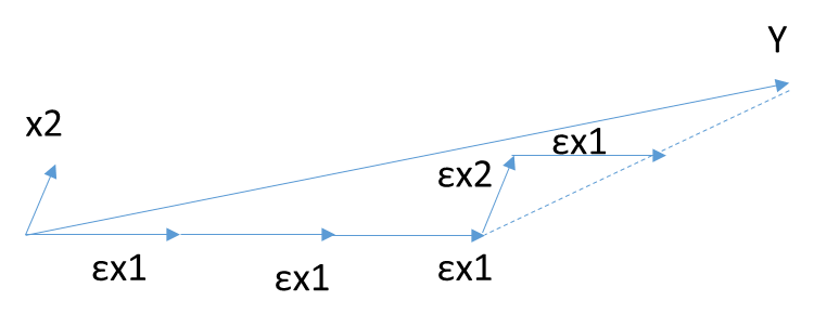
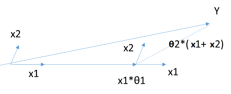
Before introducing Least Angle Regression, let ’s look at two preliminary algorithms:

(Unfinished)

4.1 Forward Selection Algorithm

4.2 Forward Stagewise Algorithm

4.3 Least Angle Regression Algorithm (LARS)

5. Conclusion

Reference:

• LEAST ANGLE REGRESSION By BRADLEY EFRON
• [web](